The task of optimizing.

Imagine we are space explorers. We are a board our craft, far from home, hyper-galactic vagabonds in pursuit of life and meaning. We land on an exoplanet, slimy and cold, and our sensors detect some weird signals and obscure measurements, and something inside of us starts to shiver. Might this be real? Have we found life?

We send out our spectrophotometer, accelerator, and low-resolution camera. All are rudimentary devices, sturdy and reliable, able to cope with the harsh environmental conditions. We soon get some measurements back to our vessel. We're excited. Our screen blinks once, and data begins to pour. 

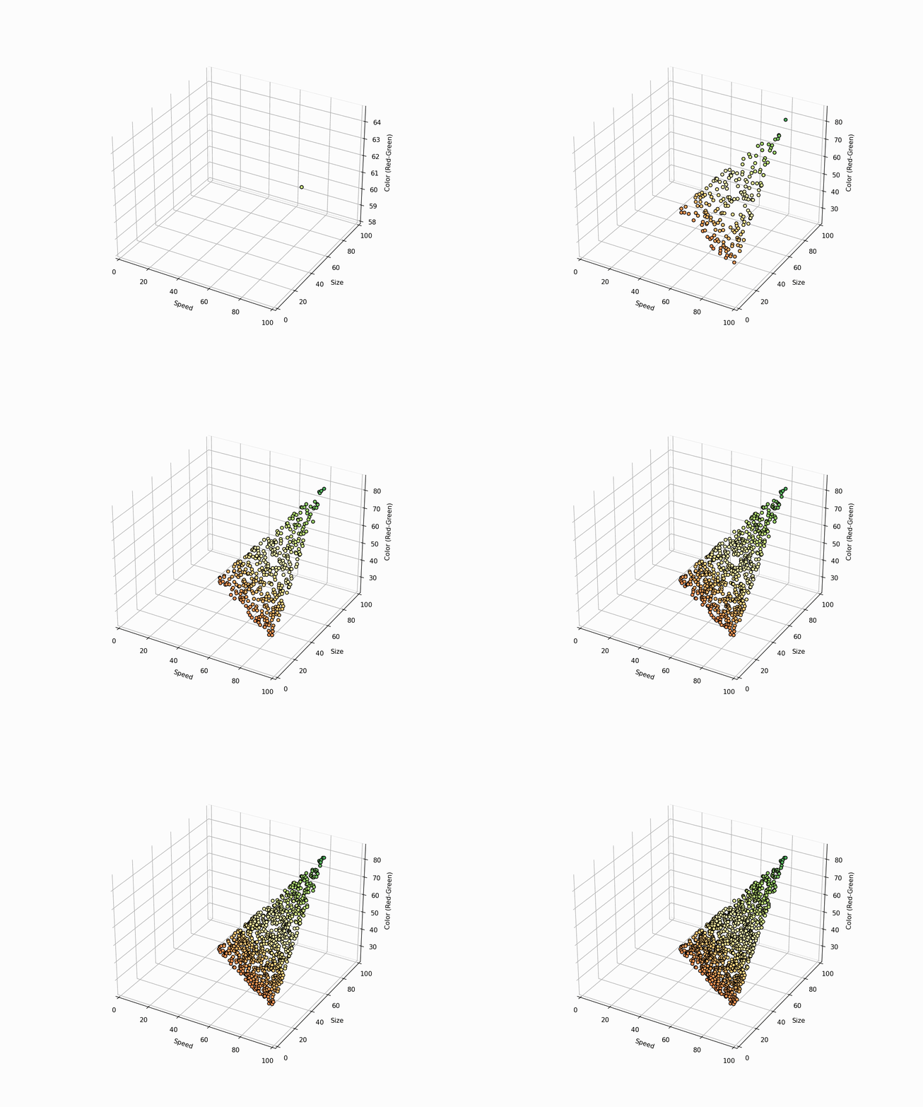
The dots aggrate. strangly.

We used our devices to form a 3D space. The axes are the Size of an object, the Speed at which the object moves, and the object's color.

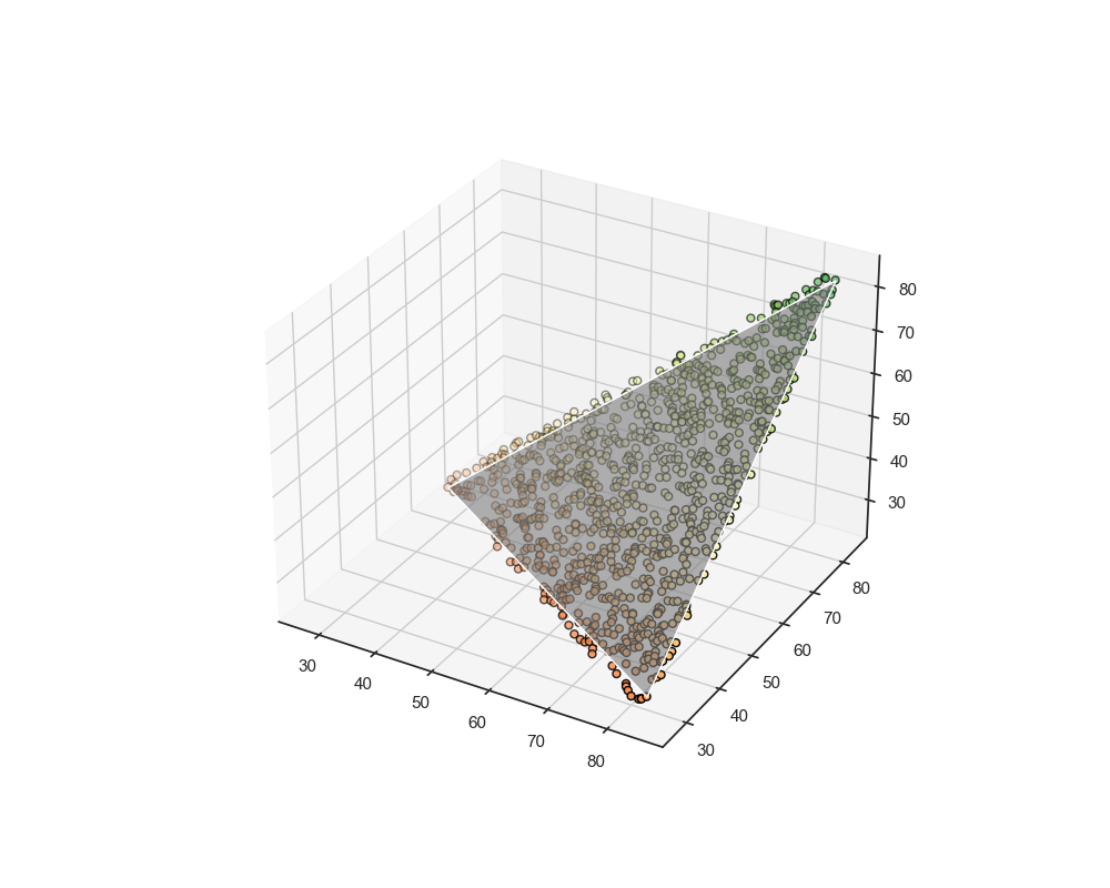
There is an order in this distribution. It is by no means random and seems to be triangular? And flat? Why would that be the case? 

This weird shape might be because of the distributions phenotypes tend to take to achieve optimality in task performance. What I mean by that is the Parato distribution aimed at optimizing task allocation.    

But what is the parato front in this context? Why would that suggest the "planarity" of the data representation? The Pareto principle indicates that resources tend to be distributed in an efficient front between the tasks needed to be performed.

This assumption indicates that when surveying organisms living in the phenotypic space they inhabit, we actually see them in a tradeoff between the tasks they need to perform. In the context of our measurements shown above, we are actually surveying the task space.

Are our measurements arbitrary? After all, we just happened to have three sensors, and our phenotypes conveniently fell on these axes. This is a valid counterargument. However, it's essential to recognize that these tasks not only guide the distribution of individuals but also shape the multi-gene networks responsible for producing specific phenotypes. Because these networks are such crucial organizing modulating factors, most measurements will likely capture something resembling this principle, irrespective of the sensors we use.

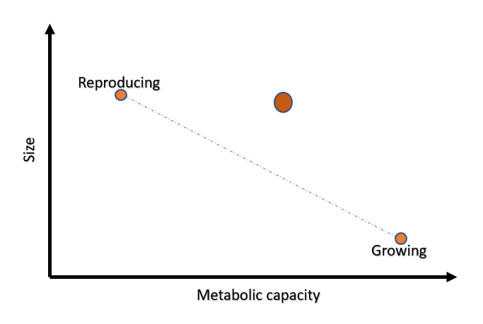
So, why is the distribution flat? Picture this: an organism striving to balance two critical tasks - growth and reproduction. In this scenario, we measure just two traits: Size and Metabolic rate. The axis spanning these traits would reveal the distributions aimed at these specific tasks.

Surveying the data, we'd likely spot two distinct phenotypic archetypes:

1. Big and slow-metabolizing cells focused on reproduction.

2. Small and fast-metabolizing cells geared towards growth.

Most individuals would be situated somewhere along the axis connecting these two archetypes, migrating between the two depending on environmental or genetic factors.

But what about outliers? Let's say an organism emerges with an atypical phenotype (represented by a prominent orange dot) situated above this axis. Unfortunately, this organism's odds of survival are slim. The reason? Relentless evolutionary pressure. For every point above (or below) our established axis, another organism better adapted to the environment and more adept at balancing growth and reproduction will outcompete and eventually outlive the outlier.

Armed with this information, we send our high-resolution camera out to the archetypes, trying to understand something about the phenotypes involved, but again, a tradeoff. Our high-resolution camera can only take three pictures before it is destroyed, so we decided to capture the archetypes and retrieve a vivid image.

The image reveals three archy phenotypes:

• Green. big, quick, and strong.

• Red, slow, and big.

• Red, but small and quick.

We, of course, know nothing about their tasks, but we can be certain these are highly optimized phenotypes aimed at specifically tackling those tasks. In fact, as the space is so well-defined, we begin to wonder if we need all three probes to accurately describe the phenotypes?

let’s plot each indvidual paremeter idepenintly than the other in this ridgeplot:

They each there own distrbution portraid by the uncertinity or entropy each one contributes:

Entropy for Speed: 2.5082
Entropy for Size: 2.3607
Entropy for Color: 2.4627

But let’s say we want to guess the one measuerment from another. For this situation let’s say we are only intrested in creatures above the size of 65. The residual entropy left is:

Entropy for Speed: 2.5055
Entropy for Size: 1.2921
Entropy for Color: 2.3474

what happend here is that one measuerment (speed) in which we lowerd the entropy by cutting most of the sample didn’t reduced our uncertinint or contributed much Mutual Information beacuse large aliens (>65) can still be in many states.

But what if we turnacte another paremter, let’s say color (>65) our new entropy would be:

Entropy for Speed: 1.3713
Entropy for Size: 1.1463
Entropy for Color: 1.1892

Indicating that by knowing the color and size of an alien we lower the uncertinity about it’s speed or gain MI about the speed by 2.5082-1.3713 = 1.1369 bits!

The reason we can actually do this is an emergent property of the Pareto front. The Pareto optimality constrains the phenotypic space, making the joint probability distribution of the data more predictable. This is no mere coincidence. Biologically, there's an imperative for organisms to operate within a constrained, optimized space. Just as in data compression, where the essence of a large data set is captured in a lower dimension without significant loss of information, biology too has evolved to occupy a compact, reproducible niche in multi-dimensional space. This efficiency allows for greater adaptability, resilience, and reproduction, ensuring the propagation of life even in the vast complexities of the universe.